March 26, 2022|cheat sheet|

how to crack the mystery of the mighty DAX.

This article is complementing the blog post how to swiftly take over Power Query with the help of some useful gear. It shall act as a cheat sheet for logic and code written in Power BIs DAX. It is not supposed to cover each and every function and neither tries it to be anywhere close to a full documentation. Instead, it provides information, explanations and examples based on issues I have encountered myself either in my daily work or in community forums like community.powerbi.com or stackoverflow.com. By the way, if you need some proper sample data to try out some of the code snippets from here, have a look into how to add adventureworks sample to azure sql database.

table of content.

1. Filter on the result of aggregate functions – “sql having clause”
2. Create ranks and indexes with calculated columns
3. Mark or get the second highest value or second latest date for a group
4. Get the max/min for a measure per group
5. Create ranks and indexes dynamically with measures
6. Find out the value appearing the most across several columns
7. Display values of large numbers with different unit abbreviations
8. Return the corresponding value for the max/min of a measure per group
9. Calculate the date difference between rows over the whole table or grouped by a status
10. Retrieve and display the value of the next row within a group
11. Grouping in DAX with AllExcept or ALL + Values – “sql group by clause”
12. Count rows meeting different conditions
13. Calculate the most frequent value in a column / return the top value for a certain measure
14. Show 0 instead of BLANKs in measure
15. Retrieve start of week date / end of week date
16. Check if values of one column exist in another column
17. Calculations with disconnected tables (without relationships)
18. Count occurrence of attributes per occurrence of another attribute (calculated table)
19. Create a Running Total measure
20. Create a rolling window / moving average measure
21. Count how many times a condition over a rolling window is met
22. How to retrieve the time from a datetime column

1. Filter on the result of aggregate functions – “sql having clause”

This one is typically needed for analytical questions like:

“count all distinct customers that have had sales turnover greater than $1,000,000 over the last three months”
“count all distinct sales representatives that gained average sales revenues greater than $5,000 per week over the last quarter”
“count all distinct employees that have had less than 5 sick days during the last year”

Example:
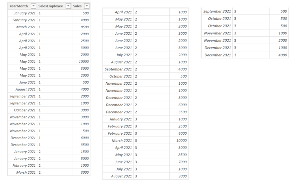
We have three sales employees in our organisation that have the following sales transactions:

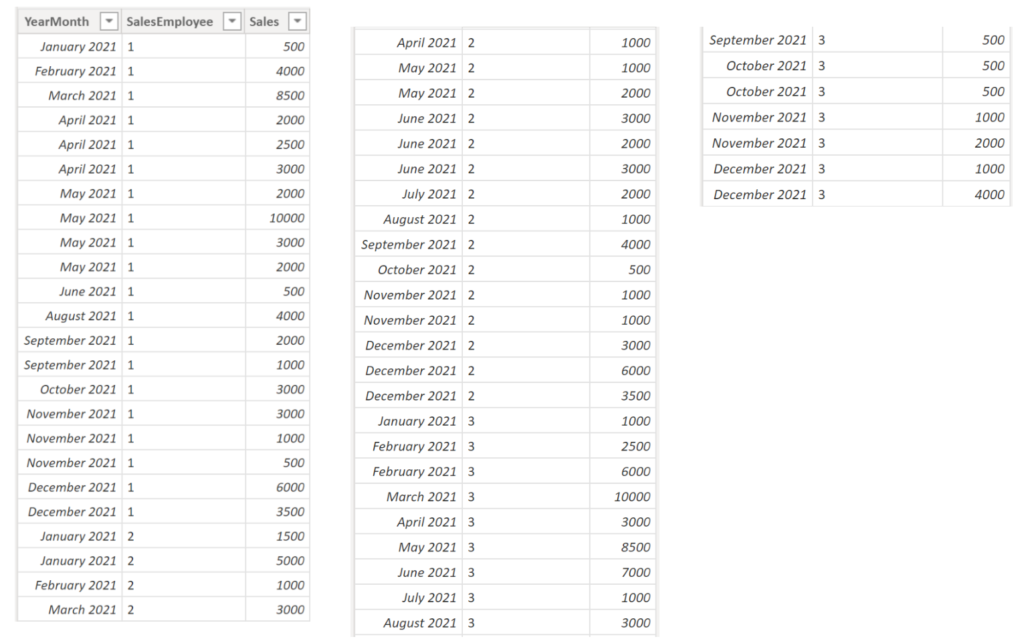
We would like to know, how many of our sale representatives achieved more than $3,000 in sales. Here the DAX code for the measure:

Measure = 
CALCULATE (
    DISTINCTCOUNT ( 'Table'[SalesEmployee] ),
    FILTER (
        VALUES ( 'Table'[SalesEmployee] ),
        CALCULATE ( SUM ( 'Table'[Sales] ) ) > 3000
    )
)

The powerful thing is that you do not need to specify the context filter in the measure. It will calculate it itself depending on what filters are applied in the visual. For instance, if we’d like to know how many of our sales people achieved more than $3,000 overall, then obviously three (namely all of them) shall be returned.
However, if we’d like to find out how many of them pulled in more than $3,000 in each month, then the measure unfolds its real usefulness:

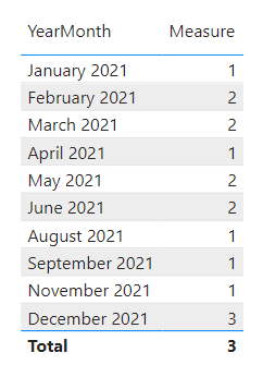
You could use the same measure even with categories, products, customers etc. and there is nothing you need to change in the DAX. It is very easy to modify the threshold in the measure, too. Here the generic code:

Measure = 
CALCULATE (
    AGGREGATEFUNCTION ( 'TableName'[ColumnName] ),
    FILTER (
        VALUES ( 'TableName'[ColumnName] ),
        CALCULATE ( AGGREGATEFUNCTION ( 'TableName'[ColumnName] ) ) > threshold
    )
)

2. Create ranks and indexes with calculated columns

Rank- and Index columns are useful not only for creating a natural order in your table, but also as a prerequisite in many other use cases.

Example:
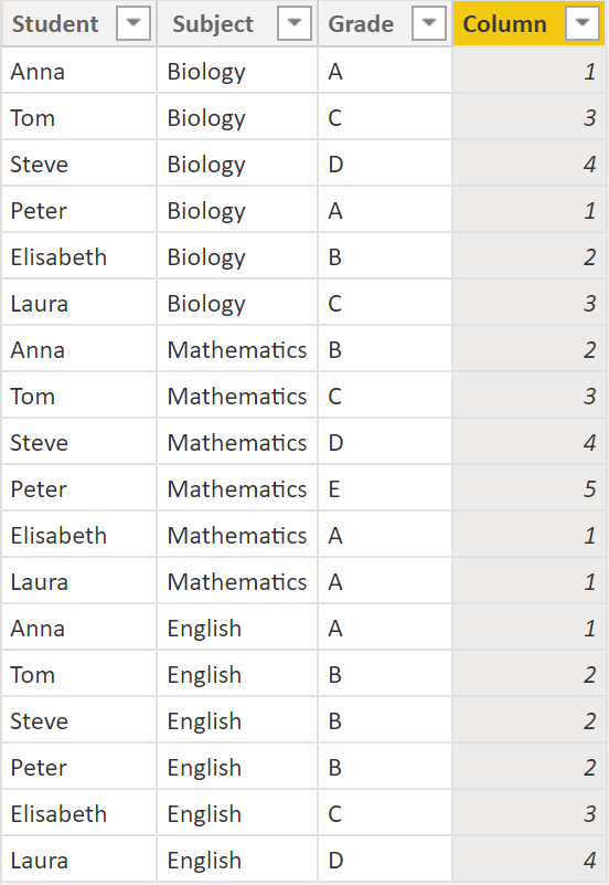
We have 6 students that all took exams in Biology, Mathematics and English with the following grades:

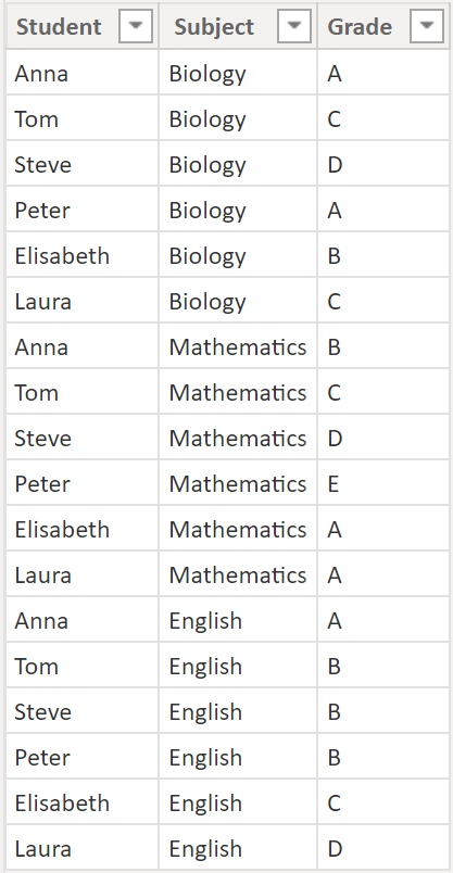
We would like to rank them on their grades per subject. Here the DAX:

Column = 
RANKX ( 
    FILTER ( 
        Table, 
        Table[Subject] = EARLIER ( Table[Subject] )
    ),
    Table[Grade],
    , ASC
    , DENSE
)

Result:

The Filter part in the DAX does the grouping (in our case per Subject). Table[Grade] is responsible for the value of the rank, ASC specifies the direction of the counting (upwards) and DENSE determines the behaviour for ties (alternative: SKIP).

Here the generic code:

Column = 
RANKX ( 
    FILTER ( 
        'TableName', 
        'TableName'[GroupingColumn] = EARLIER ( 'TableName'[GroupingColumn] )
    ),
    'TableName'[RankingColumn],
    , [ASC/DESC]
    , [DENSE/SKIP]
)

3. Mark or get the second highest value or second latest date for a group

Create a calculated column which marks each row that is the second highest for a certain group.

Example:
We have three sales employees in our organisation that have the following sales transactions:

We would like to know which of the sales for each employee was the second highest. The DAX code for the measure is as follows:

Measure = 
VAR _maxSale = 
CALCULATE ( 
    MAX ('Table'[Sales] ), 
    ALLEXCEPT ('Table','Table'[SalesEmployee] ) 
)
RETURN
CALCULATE ( 
    MAX ('Table'[Sales] ), 
    ALLEXCEPT ('Table','Table'[SalesEmployee] ), 
    'Table'[Sales] < _maxSale 
)

If you’d like to have a flag in a calculated column (for instance to be able to use it in a filter or slicer), you can use this DAX:

Calculated Column = 
VAR _maxSale = 
CALCULATE ( 
    MAX ('Table'[Sales] ), 
    ALLEXCEPT ('Table','Table'[SalesEmployee] ) 
)
VAR _secondMaxSale = 
CALCULATE ( 
    MAX ('Table'[Sales] ), 
    ALLEXCEPT ('Table','Table'[SalesEmployee] ), 
   'Table'[Sales] < _maxSale )
RETURN 
IF ( 'Table'[Sales] = _secondMaxSale, 1, 0 )

Result:

Generic Measure:

Measure = 
VAR _maxValue = 
CALCULATE ( 
    MAX ('Table'[ValueColumn] ), 
    ALLEXCEPT ('Table','Table'[GroupingColumn] ) 
)
RETURN
CALCULATE ( 
    MAX ('Table'[ValueColumn] ), 
    ALLEXCEPT ('Table','Table'[GroupingColumn] ), 
    'Table'[ValueColumn] < _maxValue
)

4. Get the max/min for a measure per group

This one is typically needed for analytical questions like:

“For each month, get the highest average amount that a customer spent”
“For each year, get the minimum amount of (the sum of) sick days that an employee had”
“For each month, get the highest accumulated sales that an employee achieved”

Example:
We have three sales employees in our organisation that have the following sales transactions:

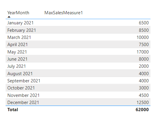
We would like to find out the maximum amount (of the sum) of sales over all employees per month. In more simple words: For each month, what was the highest accumulated sales that an employee achieved. Note, here we are not interested in who this employee was, but instead how much the employee sold. There are many ways to solve this and I will show two different ones. Since it is a two step process, we first need to have a measure in place giving us back the sum of sales:

SalesMeasure = SUM ( Table[Sales] )

Option 1
Measure:

MaxSalesMeasure1 = 
VAR _helpTable = 
SUMMARIZE ( 
    ALLEXCEPT ('Table', Table[YearMonth]), 
    'Table'[SalesEmployee], 
    "Measure", [SalesMeasure] 
)
RETURN
CALCULATE ( MAXX ( _helpTable , [Measure] ) )

Result:

Generic Measure:

Measure = 
VAR _helpTable = 
SUMMARIZE ( 
    ALLEXCEPT ('Table', Table[GroupingColumn]), 
    'Table'[SummaryColumn], 
    "Measure", [Measure] 
)
RETURN
CALCULATE ( [MAXX, MINX] ( _helpTable , [Measure] ) )

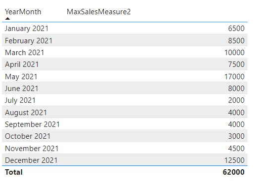
Option 2
Measure:

MaxSalesMeasure2 = 
MAXX ( VALUES ( SalesTable[SalesEmployee] ), [SalesMeasure] )

Result:

Generic Measure:

Measure = [MAXX, MINX] ( VALUES ( Table[SummaryColumn] ), [Measure] )

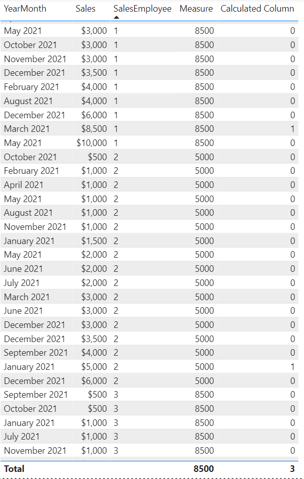
While Option 2 is way less complex than Option 1 and thus should also give performance benefits, the alternatives do differ when comparing them on a more detailed level. See Option 1 on the left and Option 2 on the right:

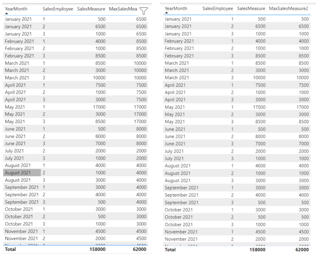
As you can see Option 1 still shows the maximum per group whereas Option 2 just displays the same as the SalesMeasure. This is because Option 1 contains a “hard” group by on YearMonth as opposed to Option 2.
Very nice, now we know the highest amount, but who was that star employee in each month? Have a look into 8. Return the corresponding value for the max/min of a measure per group to find out how we constructed that measure:

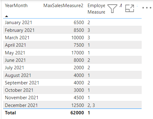
5. Create ranks and indexes dynamically with measures

As seen in the first ranks and indexes example, ranks can be added as a calculated column. This way the indexes and ranks will not change when applying filters. Here the walkthrough.

Example:
We have 6 students that all took exams in Biology, Mathematics and English with the following grades:

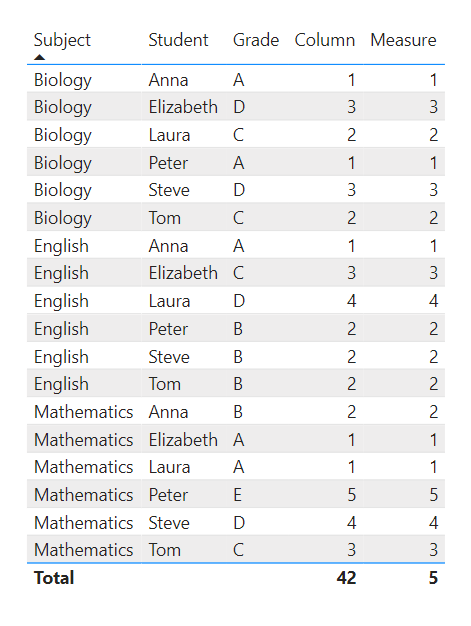
In order to find out the ranking per subject, we created a calculated column like this:

But when trying to compare only a subset of the dataset, the ranks stay static. I.e. when comparing Tom and Laura, this is what we get:

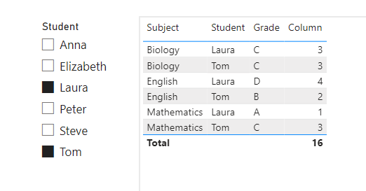
Let’s, create a Measure that dynamically adjusts to filters and slicers:

Measure = 
RANKX(
    ALLSELECTED ( Table ),
    CALCULATE ( 
        MAX ('Table'[Grade] ), 
        MAX (Table[Subject] ) = Table[Subject]
    ), 
    , ASC
    , DENSE 
) -1

Result including the calculated column:

Result with a slicer:

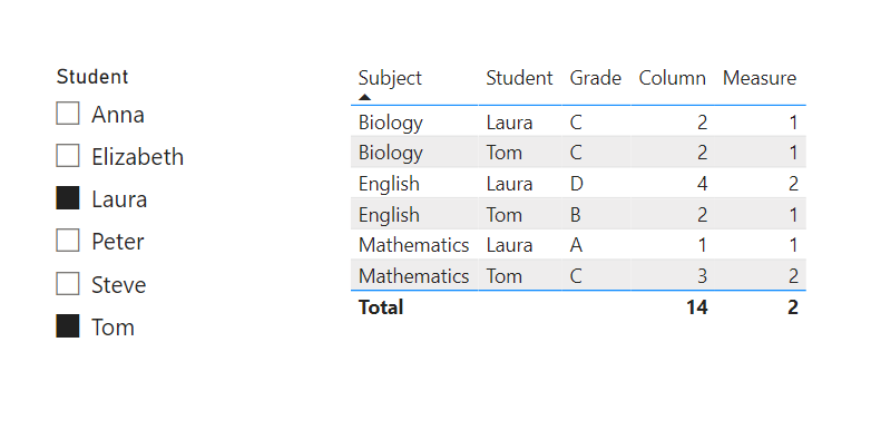
Generic Measure:

Measure = 
RANKX(
    ALLSELECTED ( TableName ),
    CALCULATE ( 
        MAX ('TableName'[RankingColumn] ), 
        MAX (TableName[GroupingColumn] ) = TableName[GroupingColumn]
    ), 
    , [ASC/DESC]
    , [DENSE/SKIP]
) -1

6. Find out the value appearing the most across several columns

Example:
We have three columns in place, each having several values:

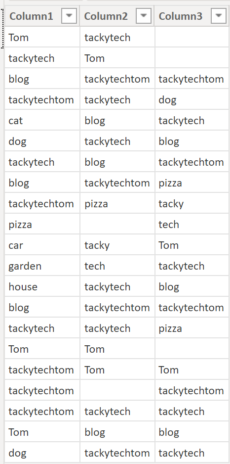
We’d like to know, which of these values occurs most often across all three columns. The solution firstly uses a union over all three columns resulting in all values being stored in one column. After, we group by each of the values including a count per value. Then we return the maximum count on which we are able to return the corresponding value.

Measure:

Measure = 
VAR _helpTable1 =
UNION ( 
        SELECTCOLUMNS( 
            RandomWordsTable, 
           "Value", RandomWordsTable[Column1]),
        SELECTCOLUMNS( 
            RandomWordsTable, 
           "Value", RandomWordsTable[Column2]),
        SELECTCOLUMNS ( 
            RandomWordsTable, 
            "Value", RandomWordsTable[Column3] )
)

VAR _helpTable2 =
GROUPBY ( 
    _helpTable1,
    [Value], "NameCountAll", COUNTX ( CURRENTGROUP(), [Value] ) 
)

VAR _maxCount =
MAXX (_helpTable2,  [NameCountAll])

RETURN
CALCULATE ( MINX ( FILTER ( _helpTable2,  [NameCountAll] = _maxCount ), [Value] ) )

Result:

Generic Measure:

Measure = 
VAR _helpTable1 =
UNION ( 
        SELECTCOLUMNS( 
            TableName, 
           "Value", TableName[Column1]),
        SELECTCOLUMNS( 
            TableName, 
           "Value", TableName[Column2]),
        SELECTCOLUMNS ( 
            RandomWordsTable, 
            "Value", TableName[Column3] )
)

VAR _helpTable2 =
GROUPBY ( 
    _helpTable1,
    [Value], "NameCountAll", COUNTX ( CURRENTGROUP(), [Value] ) 
)

VAR _maxCount =
MAXX (_helpTable2,  [NameCountAll])

RETURN
CALCULATE ( MINX ( FILTER ( _helpTable2,  [NameCountAll] = _maxCount ), [Value] ) )

7. Display values of large numbers with different unit abbreviations

When numbers in a column or a measure differ significantly, you might want to define specific unit abbreviations like M for millions or k for thousands. Sometimes you may even need different abbreviations for the same column. Here comes a possible solution on this matter.

Example:
We have the following two columns and we’d like to translate each of the numbers of the Value column to an abbreviated form:

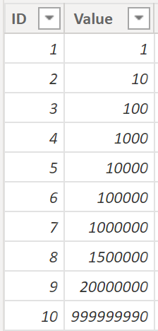
Calculated Column:

TranslatedColumn = 
SWITCH (
    TRUE,
    [Value] < 1000, FORMAT ( [Value],"Currency" ),
    [Value] < 100000, FORMAT ( DIVIDE ( [Value], 1000 ), "Currency" ) & "K",
    FORMAT ( DIVIDE ( [Value], 1000000 ), "Currency" ) & "M"
)

Result:

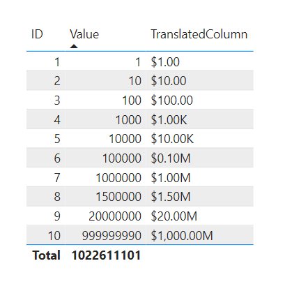
You can use the same code snippet for a measure as well. In this example, we use the ValueSum measure which equals the sum of the Value column:

TranslationMeasure = 
SWITCH (
    TRUE,
    [ValueSum] < 1000, FORMAT ( [ValueSum],"Currency" ),
    [ValueSum] < 100000, FORMAT ( DIVIDE ( [ValueSum], 1000 ), "Currency" ) & "K",
    FORMAT ( DIVIDE ( [ValueSum], 1000000 ), "Currency" ) & "M"
)

Result:

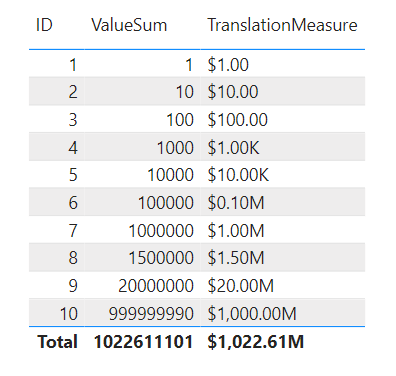
Generic Measure or Calculated Column:

ColumnOrMeasure = 
SWITCH (
    TRUE,
    [ColumnOrMeasure] < 1000, FORMAT ( [ColumnOrMeasure],"Currency" ),
    [ColumnOrMeasure] < 100000, FORMAT ( DIVIDE ( [ColumnOrMeasure], 1000 ), "Currency" ) & "K",
    FORMAT ( DIVIDE ( [ColumnOrMeasure], 1000000 ), "Currency" ) & "M"
)

8. Return the corresponding value for the max/min of a measure per group

This one is typically needed for analytical questions like:

“For each month, which customers had the highest average amount spent”
“For each year, which employees had the minimum amount of (the sum of) sick days”
“For each month, who had the highest accumulated sales”

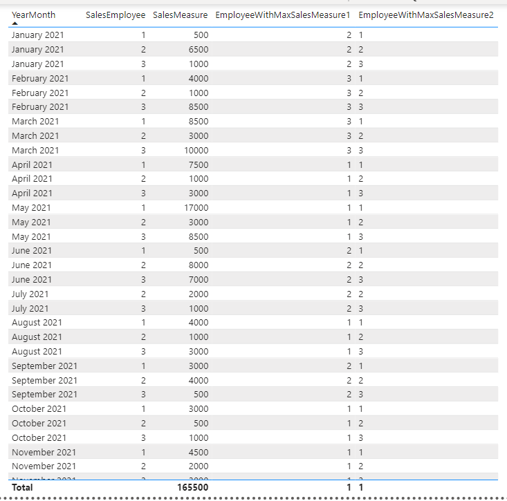
Example:
We have three sales employees in our organisation that have the following sales transactions:

We would like to find out which sales employee had the maximum amount (of the sum) of sales per month. In more simple words: For each month, what who sold the most. Note, here we are not interested in how much this employee sold for, but instead who the employee was. There are many ways to solve this and I will show two different ones. Since it is a two step process, we first need to have a measure in place giving us back the sum of sales:

SalesMeasure = SUM ( Table[Sales] )

Option 1
Measure:

EmployeeWithMaxSalesMeasure1 = 
VAR _helpTable = 
SUMMARIZE ( 
    ALLEXCEPT ('SalesTable', SalesTable[YearMonth]), 
    'SalesTable'[SalesEmployee], 
    "Measure", [SalesMeasure] 
)
VAR _maxMeasure = CALCULATE ( MAXX ( _helpTable , [Measure] ) )
RETURN
CALCULATE ( 
    MAX ( 'SalesTable'[SalesEmployee] ), 
    FILTER ( _helpTable, [Measure] = _maxMeasure )
)

Result:

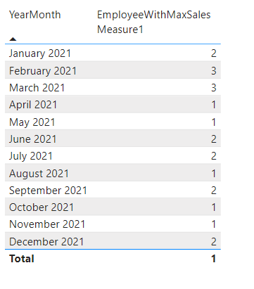
Generic Measure:

Measure = 
VAR _helpTable = 
SUMMARIZE ( 
    ALLEXCEPT ('Table', Table[GroupingColumn]), 
    'Table'[SummaryColumn], 
    "Measure", [Measure] 
)
VAR _maxMeasure = CALCULATE ( MAXX ( _helpTable , [Measure] ) )
RETURN
CALCULATE ( 
    MAX ( 'Table'[SummaryColumn] ), 
    FILTER ( _helpTable, [Measure] = _maxMeasure )
)

Option 2
Measure:

EmployeeWithMaxSalesMeasure2 = 
CONCATENATEX ( 
    TOPN ( 
        1, 
        VALUES ( SalesTable[SalesEmployee] ), 
        [SalesMeasure] 
    ), 
    SalesTable[SalesEmployee], ", "
)

Result:

Generic Measure:

Measure = 
CONCATENATEX ( 
    TOPN ( 
        1, 
        VALUES ( Table[SummaryColumn] ), 
        [Measure] 
    ), 
    Table[SummaryColumn], ", "
)

While Option 2 is way less complex than Option 1 and thus should also give performance benefits, Option 2 even shows multiple sales employee if there are draws. The alternatives do differ when comparing them on a more detailed level though. See Option 1 with EmployeeWithMaxSalesMeasure1 on the left and Option 2 with EmployeeWithMaxSalesMeasure2 on the right:

As you can see Option 1 still shows the maximum per group whereas Option 2 just displays the same as the actual SaoesEmployee. This is because Option 1 contains a “hard” group by on YearMonth as opposed to Option 2.
Very nice, now we know who that star employee in each month was, but how much was the actual amount? Have a look into 4. Get the max/min for a measure per group to find out how we constructed that measure:

9. Calculate the date difference between rows over the whole table or grouped by a status

A classic one. We would like to calculate the number of days one status lasted until it switched to the next status – either over the whole table or by a group.

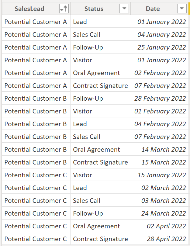
Example:
We have three sales leads in the following table that went through a sales funnel. The table shows for each sales lead on which date they entered a specific status. We would like to know how many days a sales lead spent in the respective status.

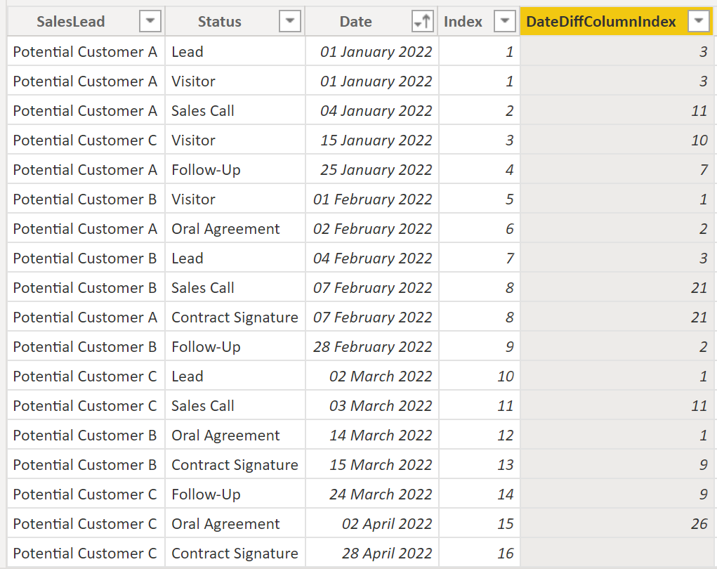
To calculate the difference per row, we need to specify the order on how DAX shall run through the table. For this we must provide a rank / index column. You can look into this part to learn more about how to create ranks / indexes. We start with an index without a grouping:

Index = 
RANKX ( 
    'SalesLead',
    'SalesLead'[Date],
    , ASC
    , DENSE
)

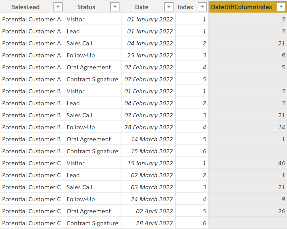
On the base of this index, we can now create the DateDiffColumnIndex:

DateDiffColumnIndex = 
DATEDIFF (
   'SalesLead'[Date],
    CALCULATE (
        MAX ( 'SalesLead'[Date] ),
        FILTER ( 'SalesLead', 'SalesLead'[Index] = EARLIER ( 'SalesLead'[Index] ) + 1 )
    ),
    DAY
)

Result:

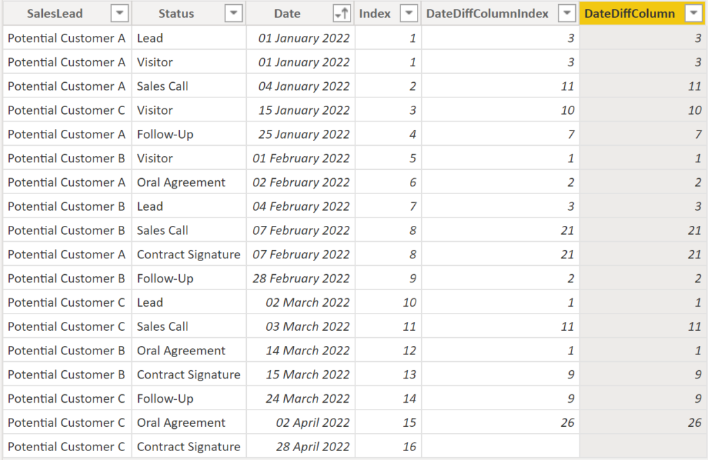
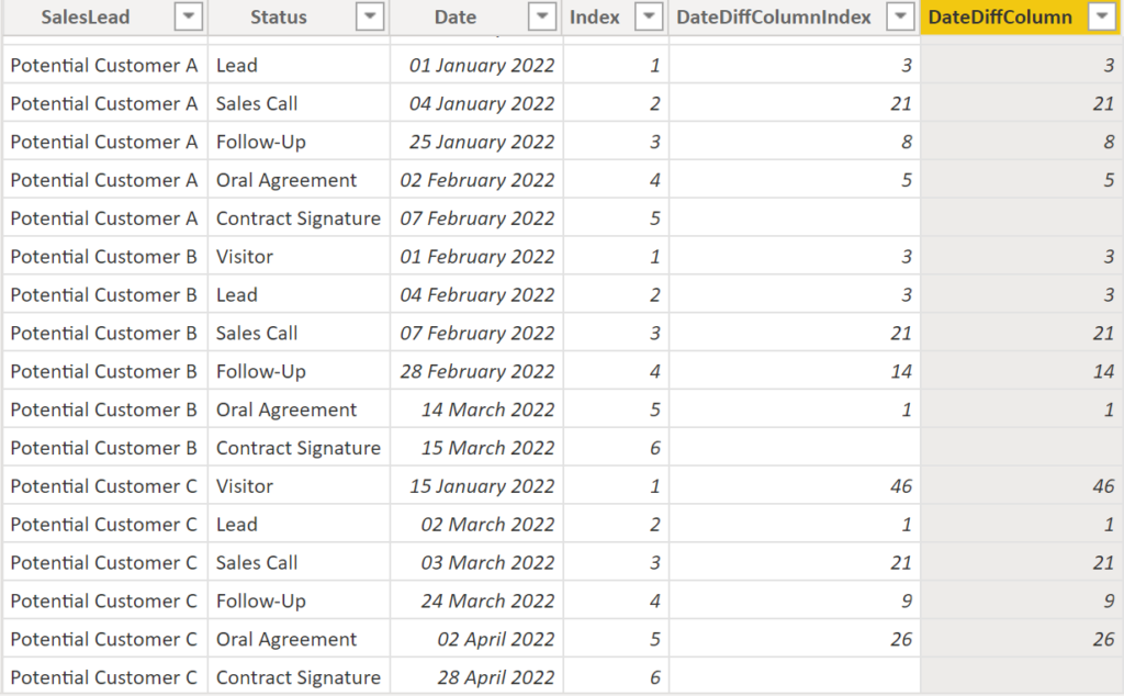
Since there is already a natural order on the table, you would not necessarily need to create an index column to retrieve the result above.
This measure will give you the same result:

DateDiffColumn = 
DATEDIFF (
   'SalesLead'[Date],
    CALCULATE (
        MIN ( 'SalesLead'[Date] ),
        FILTER ( 'SalesLead', 'SalesLead'[Date] > EARLIER ( 'SalesLead'[Date] )  )
    ),
    DAY
)

Result:

Obviously, the solution above does not provide too much of a value since it ignores the grouping per SalesLead. Let’s add the SalesLead grouping to the index.

Index = 
RANKX ( 
    FILTER ( 
        'SalesLead', 
        'SalesLead'[SalesLead] = EARLIER ( 'SalesLead'[SalesLead] )
    ),
    'SalesLead'[Date],
    , ASC
    , DENSE
)

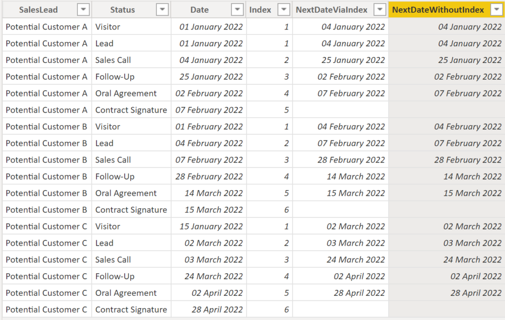
Let’s also add the grouping on SalesLead to DateDiffColumnIndex:

DateDiffColumnIndex = 
DATEDIFF (
   'SalesLead'[Date],
    CALCULATE (
        MAX ( 'SalesLead'[Date] ),
        FILTER ( 'SalesLead', 'SalesLead'[Index] = EARLIER ( 'SalesLead'[Index] ) + 1 ),
        FILTER ( 'Sale...sLead', 'SalesLead'[SalesLead] = EARLIER ( 'SalesLead'[SalesLead] ) )
       
    ),
    DAY
)

Result:

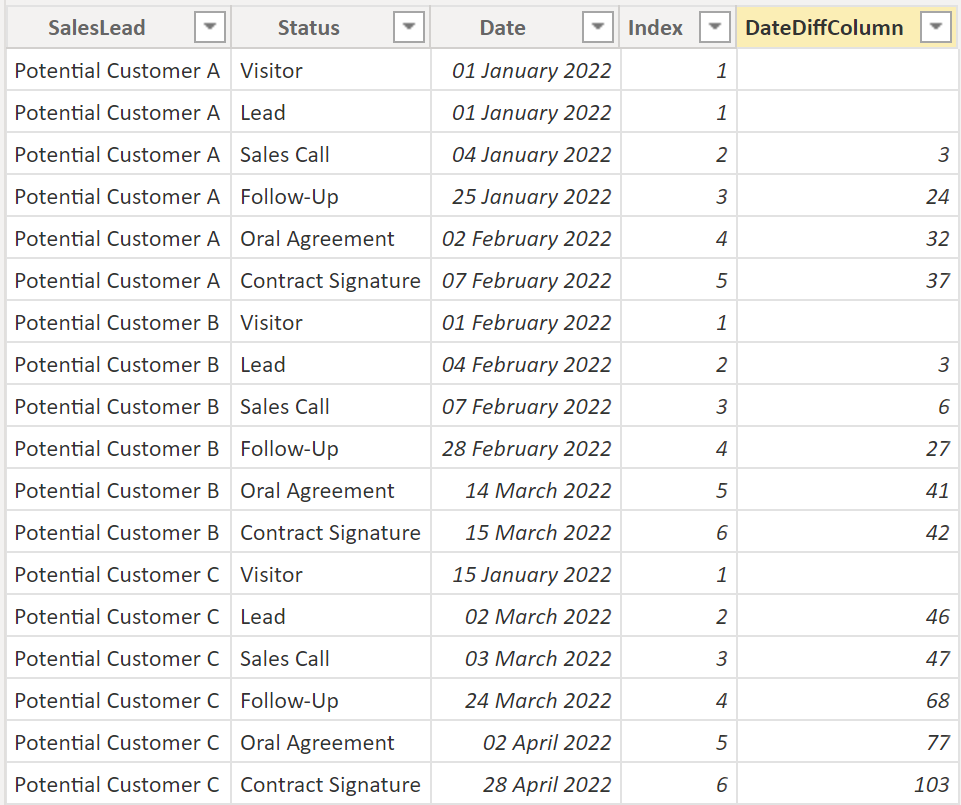
Likewise we can tweak the DateDiffColumn to include the grouping column SalesLead, too:

DateDiffColumn = 
DATEDIFF (
   'SalesLead'[Date],
    CALCULATE (
        MIN ( 'SalesLead'[Date] ),
        FILTER ( 'SalesLead', 'SalesLead'[Date] > EARLIER ( 'SalesLead'[Date] )  ),
        FILTER ( 'SalesLead', 'SalesLead'[SalesLead] = EARLIER ( 'SalesLead'[SalesLead] ) )
    ),
    DAY
)

Result:

So essentially, there are multiple ways on how to solve this matter. Depending on whether you are having an index column in place or not, here the generic DAX for the calculated columns:

DateDiffColumnWithIndex = 
DATEDIFF (
   'TableName'[RankingColumn],
    CALCULATE (
        MAX ( 'TableName'[RankingColumn] ),
        FILTER ( 'TableName', 'TableName'[Index] = EARLIER ( 'TableName'[Index] ) + 1 ),
        FILTER ( 'TableName', 'TableName'[GroupingColumn] = EARLIER ( 'TableName'[GroupingColumn] ) ) 
    ),
    DAY
)

DateDiffColumnWithoutIndex = 
DATEDIFF (
   'TableName'[RankingColumn],
    CALCULATE (
        MIN ( 'TableName'[RankingColumn] ),
        FILTER ( 'TableName', 'TableName'[RankingColumn]  > EARLIER ( 'TableName'[RankingColumn]  ) ),
        FILTER ( 'TableName', 'TableName'[GroupingColumn] = EARLIER ( 'TableName'[GroupingColumn] ) )
    ),
    DAY
)

Lastly, by changing the order of the attributes within the DATEDIFF function and switching the Greater-than sign to a Less-than sign, the result will be showing how long it took to switch status rather than how long the status lasted. In other words, it creates the difference between each row for a group:

DateDiffColumnWithIndex = 
DATEDIFF (
    CALCULATE (
        MAX ( 'SalesLead'[Date] ),
        FILTER ( 'SalesLead', 'SalesLead'[Date] = EARLIER ( 'SalesLead'[Date] ) - 1 ),
        FILTER ( 'SalesLead', 'SalesLead'[SalesLead] = EARLIER ( 'SalesLead'[SalesLead] ) )
    ),
   'SalesLead'[Date],
    DAY
)

DateDiffColumnWithoutIndex = 
DATEDIFF (
    CALCULATE (
        MIN ( 'SalesLead'[Date] ),
        FILTER ( 'SalesLead', 'SalesLead'[Date] < EARLIER ( 'SalesLead'[Date] )  ),
        FILTER ( 'SalesLead', 'SalesLead'[SalesLead] = EARLIER ( 'SalesLead'[SalesLead] ) )
    ),
   'SalesLead'[Date],
    DAY
)

Result:

The generic DAX:

DateDiffColumnWithIndex = 
DATEDIFF (
    CALCULATE (
        MAX ( 'TableName'[RankingColumn] ),
        FILTER ( 'TableName', 'TableName'[RankingColumn] = EARLIER ( 'TableName'[RankingColumn] ) - 1 ),
        FILTER ( 'TableName', 'TableName'[GroupingColumn] = EARLIER ( 'TableName'[GroupingColumn] ) )
    ),
   'TableName'[RankingColumn],
    DAY
)

DateDiffColumnWithoutIndex = 
DATEDIFF (
    CALCULATE (
        MIN ( 'TableName'[RankingColumn] ),
        FILTER ( 'TableName', 'TableName'[RankingColumn]  < EARLIER ( 'TableName'[RankingColumn]  ) ),
        FILTER ( 'TableName', 'TableName'[GroupingColumn] = EARLIER ( 'TableName'[GroupingColumn] ) )
    ),
   'TableName'[RankingColumn],
    DAY
)

10. Retrieve and display the value of the next row within a group

Similar to the previous part, here we would like to retrieve and display the value of the next row without doing any calculations. This can be something like stamp the row with the date of the next status.

Option 1. Create an index column and reuse it in a calculated column.

Index = 
RANKX ( 
    FILTER ( 
        'SalesLead', 
        'SalesLead'[SalesLead] = EARLIER ( 'SalesLead'[SalesLead] )
    ),
    'SalesLead'[Date],
    , ASC
    , DENSE
)

NextDateViaIndex = 
CALCULATE (
    MAX ( 'SalesLead'[Date] ),
    FILTER ( 'SalesLead', 'SalesLead'[Index] = EARLIER ( 'SalesLead'[Index] ) + 1 ),
    FILTER ( 'SalesLead', 'SalesLead'[SalesLead] = EARLIER ( 'SalesLead'[SalesLead] ) )  
)

Result:

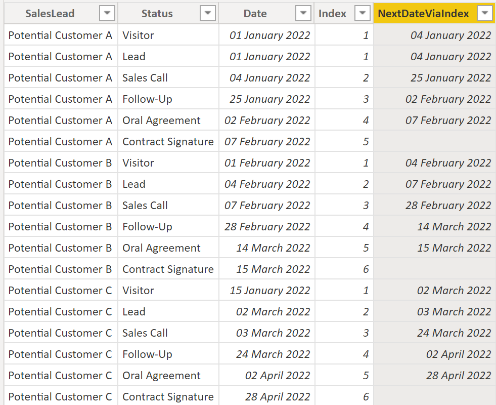
Option 2. Create a calciulated column without using an index:

NextDateWithoutIndex = 
CALCULATE (
    MIN ( 'SalesLead'[Date] ),
    FILTER ( 'SalesLead', 'SalesLead'[Date] > EARLIER ( 'SalesLead'[Date] )  ),
    FILTER ( 'SalesLead', 'SalesLead'[SalesLead] = EARLIER ( 'SalesLead'[SalesLead] ) )
)

Result:

Option 3. We can also get this information by utilizing a variable plus removing all filters except the grouping one:

NextDateWithAllExcept = 
VAR _currentDate = 'SalesLead'[Date] 
RETURN
CALCULATE ( 
    MIN ( 'SalesLead'[Date] ), 
    ALLEXCEPT ( 'SalesLead', 'SalesLead'[SalesLead] ),
    'SalesLead'[Date] > _currentDate 
)

Result:

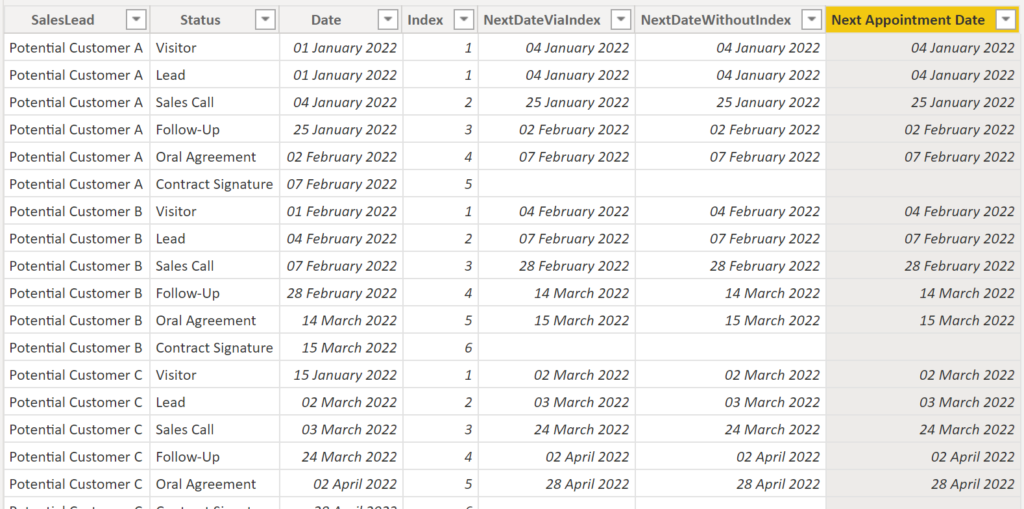
In the following, the generic code for either of the options:

NextDateViaIndex = 
CALCULATE (
    MAX ( 'TableName'[Value] ),
    FILTER ( 'TableName', 'TableName'[RankingColumn]  = EARLIER ( 'TableName'[RankingColumn]  ) + 1 ),
    FILTER ( 'TableName', 'TableName'[GroupingColumn] = EARLIER ( 'TableName'[GroupingColumn] )     )  
)

NextDateWithoutIndex = 
CALCULATE (
    MIN ( 'TableName'[Value] ),
    FILTER ( 'TableName', 'TableName'[RankingColumn]  > EARLIER ( 'TableName'[RankingColumn)  ),
    FILTER ( 'TableName', 'TableName'[GroupingColumn] = EARLIER ( 'TableName'[GroupingColumn] ) )
)

NextDateWithAllExcept = 
VAR _currentRank = 'TableName'[RankingColumn] 
RETURN
CALCULATE ( 
    MIN ( 'TableName'[Value] ), 
    ALLEXCEPT ( 'TableName', 'TableName'[GroupingColumn] ),
    'TableName'[RankingColumn] > _currentRank 
)

Note: You can return any value of the next row. However, it can be that you need to swap MIN with MAX. Likewise, you can pick the value from the previous by switching the Greater-than sign with the Less-than sign.

11. Grouping in DAX with AllExcept or ALL + Values – “sql group by clause”

Groupings in combination with aggregations are probably one of the most basic analytical use cases. There are quite a few ways of implementing it and here we’ll show you two of them!

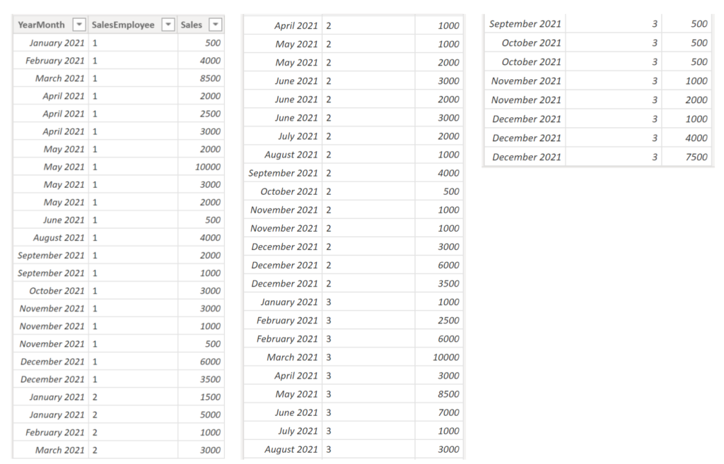
Example:
We have three sales employees in our organisation that have the following sales transactions:

We would like to find out sales grouped by SalesEmployee. Luckily, Power BI makes it easy for us by automatically applying the grouping when dragging attributes into visuals:

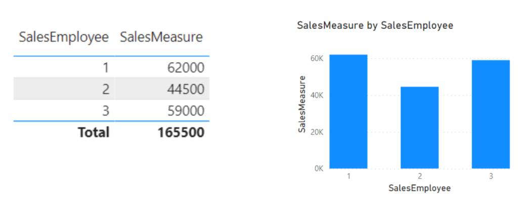
However, we sometimes still need to establish groupings in DAX, for instance to use the aggregated result further in a measure or to make the result “static”: When dragging another attribute into our table from above, the grouping is automatically applied on both SalesEmployee and the new column:

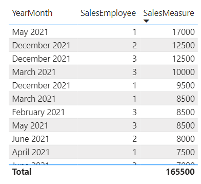
So, let’s create a DAX measure which solidifies the grouping on SalesEmployee. Here are two ways – one with ALLEXCEPT and another one with ALL + VALUES. The idea is to remove all filters from the context except the one that you’d like to group on. With that filter in place, the result is automatically grouped.

MeasureAllExcept = 
CALCULATE (
    [SalesMeasure],
    ALLEXCEPT ( SalesTable, SalesTable[SalesEmployee] )
)

MeasureAllValues = 
CALCULATE (
    [SalesMeasure],
    ALL ( SalesTable ), 
    VALUES ( SalesTable[SalesEmployee] )
)

Result:

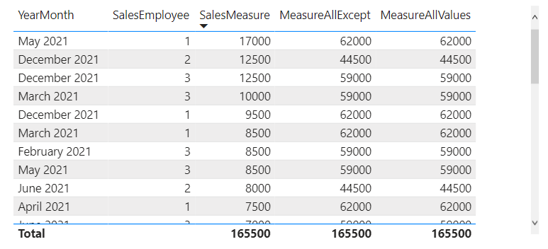
Both measure work well! However, as Marco Russo and Alberto Ferrari claim here, it is generally a better idea to use ALL + VALUES approach. Also, the ALL function can be substituted with REMOVEFILTERS. They are aliases, however, REMOVEFILTERS makes it easier to read.

The generic code for both ways:

MeasureAllExcept = 
CALCULATE (
    [Measure],
    ALLEXCEPT ( TableName, TableName[GroupingColumn] )
)

MeasureAllValues = 
CALCULATE (
    [Measure],
    ALL ( TableName), 
    VALUES ( TableName[GroupingColumn] )
)

12. Count rows meeting different conditions

This one is typically needed for analytical questions like:

“count all customers that either belong to the category “B2B” or that have a turnover larger than $1 Mio”
“count all sales representatives that either have been at the company for at least three years or “KAMs”
“count all employees that have been at the company for less than one year or still are in probation period”

Example:
To make the use case generic, we have a table with place holder conditions. Your table does not need to have Boolean values. Instead, it can be any kind of attribute that will turn into a Boolean through conditioning and filtering:

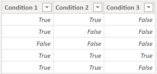
We would like to find out how many rows meet at least one of the three conditions. It is a classic use case for the OR operator. However, since PBI considers TRUE and FALSE as 1 and 0 respectively, we can create a measure utilizing this matter:

MeasureCount = 
COUNTROWS ( 
    FILTER ( 
        ConditionalTable, 
        [Condition 1] + [Condition 2] + [Condition 3] >= 1
    )
)

Result:

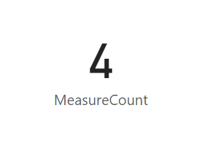
We can easily tweak the code of the measure in case our requirement changes. For instance, if we want at least two out of the three conditions to be met, then we just need to substitute the 1 with 2. If we would like to count the rows that at least have one condition to be FALSE, then we need to use the condition “<= 2“.

The generic code:

MeasureCount = 
COUNTROWS ( 
    FILTER ( 
        Table, 
        [Condition1] + [Condition2] + [Condition3] [>=, <=, >, <, =] Number
    )
)

13. Calculate the most frequent value in a column / return the top value for a certain measure

Example:
We would like to return the most common or frequent value from the below column:

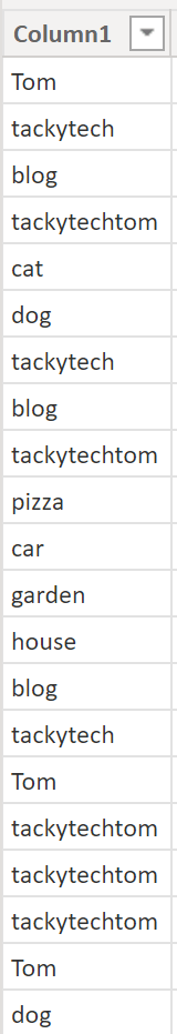
First, we need to create a count measure:

CountMeasure =
COUNT ( RandomWordsTable[Column1] )

This leads to the following result:

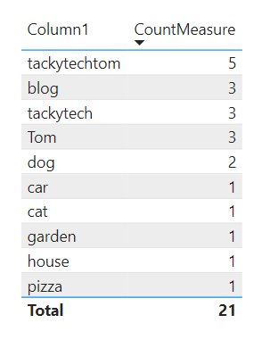
Next, we need to create the measure:

TopCountMeasure =
FIRSTNONBLANK (
    TOPN (
        1, 
        VALUES ( Table[Column1] ), 
        RANKX( ALL( Table[Column1] ), [CountMeasure] , , ASC)
    ), 
    1 
)

Result:

By the way, the CountMeasure can be of any kind of nature and does not necessarily need to be counting over a column. In fact, you can use any kind of measure and you will always return the corresponding value for it. Likewise, if you would like to return the attribute with the least value, just use DESC.

The generic code:

Measure = 
FIRSTNONBLANK (
    TOPN (
        1, 
        VALUES ( Table[Column] ), 
        RANKX( ALL( Table[Column] ), [Measure] , , [DESC/ASC] )
    ), 
    1 
)

14. Show 0 instead of BLANKs in measure

We all have been there. You created a measure that with some slicing and filtering does not show any value for some of the elements. Here a way to convert BLANKs to 0

Example:
We have 6 students that all took exams in Biology, Mathematics and English with the following grades:

We would like find out the number of times a student has had an A on the three exams.

We create the following DAX:

CountAGrades = 
CALCULATE ( 
    COUNTROWS ( StudentGradeTable ),
    StudentGradeTable[Grade] = "A" 
)

Result:

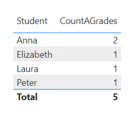
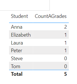
Unfortunately, all the ones that did not have an A will not appear in the table. That Power BI does not visualise the other ones is by design and has advantages, i.e. clarity and performance. If you’d like to show the other students with a 0 (instead of a blank), you could wrap the measure into an if clause. A much simpler solution is to add a 0 add the end, though:

CountAGrades = 
CALCULATE ( 
    COUNTROWS ( StudentGradeTable ),
    StudentGradeTable[Grade] = "A" 
) + 0

Result:

15. Retrieve start of week date / end of week date

If your date / calendar dimension does not have an attribute showing the date of the beginning / end of week, have a look below.

Example:
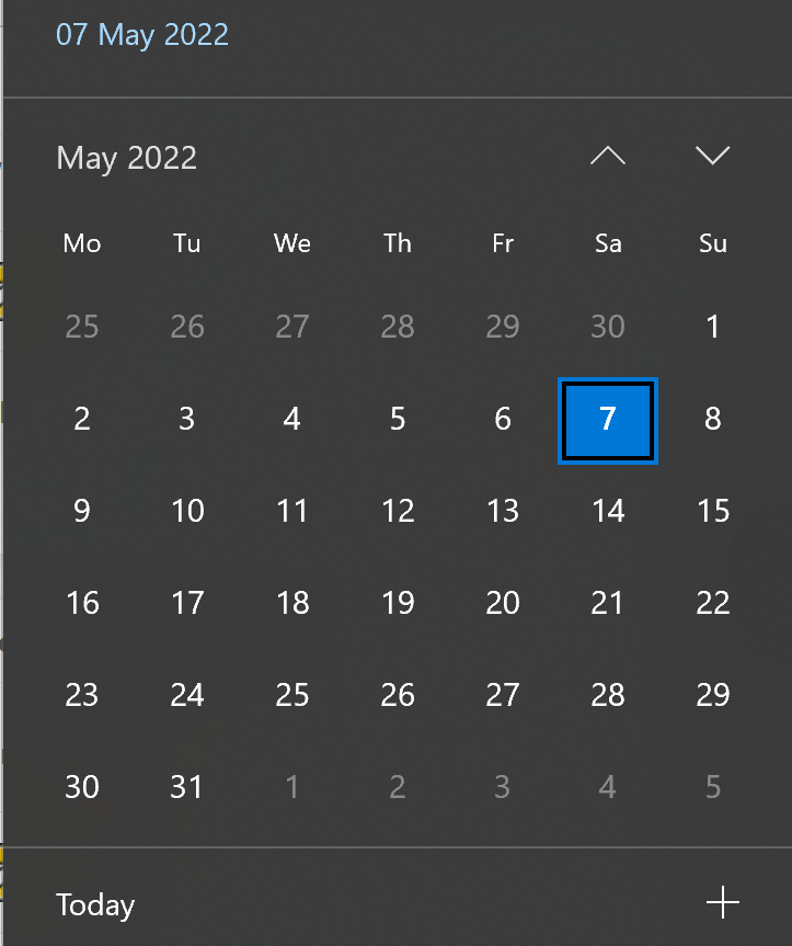
As time of writing, today’s date is the 7th of May 2022:

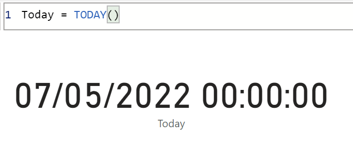
So, the beginning of that week was on Monday the 2nd of May 2022 and the end of that week was on Sunday the 8th of May 2022. Note: We follow European standard where weeks start on Mondays and end on Sundays.

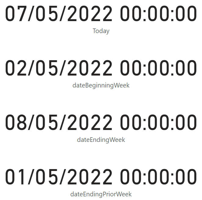
Here the DAX:

dateBeginningWeek = 
TODAY() + 1 - WEEKDAY ( TODAY(), 2 )

dateEndingWeek = 
TODAY() + 7 - WEEKDAY ( TODAY(), 2 )

dateEndingPriorWeek = 
TODAY() - WEEKDAY ( TODAY(), 2 )

Result:

Note: You can easily substitute the TODAY() function with a reference to your date column or measure.

16. Check if values of one column exist in another column

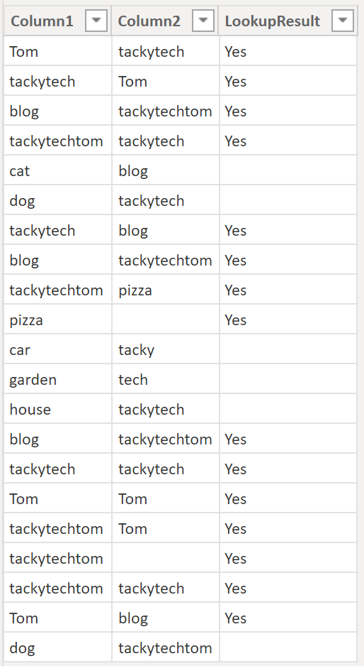
We’d like to find out for each row in column1 whether it exists in column2 – much like the Excel lookup function. The result we wanna save in a separate column (LookupResult):

Example/result:

The DAX for the calculated column LookUpResult, would look like this:

LookupResult = 
IF ( 
    CONTAINS ( 
        RandomWordsTable, 
        RandomWordsTable[Column2], 
        RandomWordsTable[Column1] 
    ), 
    "Yes", 
    BLANK()
)

Note, you can also solve this issue in Power Query.

17. Calculations with disconnected tables (without relationships)

There are cases where one needs to utilize two or more tables that do not have relationships in order to execute calculations.

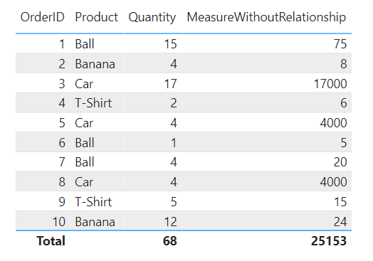
Example:

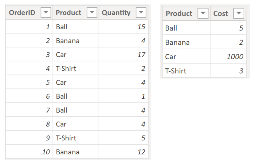
In the example above, we have two tables (left: TableA as our FactTable / right: TableB as our DimTable) without a connection. We are aiming to calculate the total costs per Order.

The DAX for the measure:

MeasureWithoutRelationship = 
SUMX ( 
    TableA, 
    TableA[Quantity] * 
    CALCULATE ( 
        VALUES ( TableB[Cost] ),
        FILTER ( 
            TableB, 
            TableB[Product] = TableA[Product] 
        ) 
    ) 
 )

Result:

The generic code:

Measure = 
[Calculation:SUMX/AVERAGEX] ( 
    FactTable, 
    FactTable[Fact] [Operator:*/-+]
    CALCULATE ( 
        VALUES ( DimTable[Attribute] ),
        FILTER ( 
            DimTable, 
            DimTable[PrimaryKey] = FactTable[ForeignKey] 
        ) 
    ) 
 )

18. Count occurrence of attributes per occurrence of another attribute (calculated table)

This one does a grouping with a count on the basis of another grouping and count. For instance, you would like to get a summary table on how many customers (attribute 1) have bought 1, 2 or 3 different products (attribute 2):

Example:

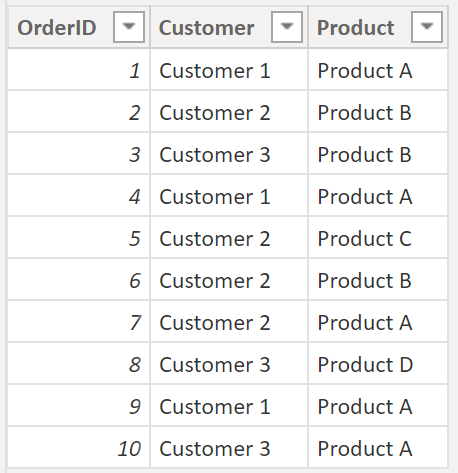
The DAX for calculated table:

New Table = 
VAR _helpTable =
SUMMARIZE (
    OrderTable,
    OrderTable[Customer],
    "Nbr of Products", DISTINCTCOUNT ( OrderTable[Product] )
)
RETURN
SUMMARIZE (
    _helpTable,
    [Nbr of Products],
    "Nbr of Customers",
    CALCULATE (
        DISTINCTCOUNT ( 'OrderTable'[Customer] ),
        FILTER (
            VALUES ( 'OrderTable'[Customer] ),
            CALCULATE ( DISTINCTCOUNT ( OrderTable[Product] ) ) = [Nbr of Products]
        )
    )
)

Result:

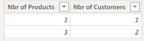
The generic code:

Table = 
VAR _helpTable =
SUMMARIZE (
    Table,
    Table[Attribute1],
    "Nbr of Attribute2", DISTINCTCOUNT ( Table[Attribute2] )
)
RETURN
SUMMARIZE (
    _helpTable,
    [Nbr of Attribute2],
    "Nbr of Attribute1",
    CALCULATE (
        DISTINCTCOUNT ( 'Table'[Attribute1] ),
        FILTER (
            VALUES ( 'Table'[Attribute1] ),
            CALCULATE ( DISTINCTCOUNT ( Table[Attribute2] ) ) = [Nbr of Attribute2]
        )
    )
)

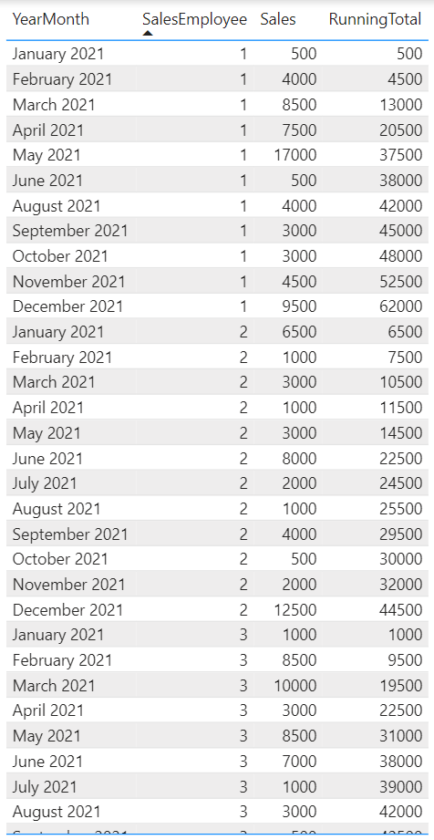
19. Create a Running Total measure

Here, we need a measure that creates a running total, often also called YearToDate.

Example:

The DAX for the measure:

RunningTotal = 
CALCULATE (
    SUM ( 'SalesTable'[Sales] ),
    DATESYTD( 'SalesTable'[YearMonth] )
)

Result:

The DATESYTD function only changes the filter context of the Date column meaning natural groupings within the graphs are not affected.

The generic code:

Measure = 
CALCULATE (
    SUM ( 'Table'[NumberColumn] ),
    DATESYTD( 'Table'[DateColumnn] )
)

20. Create a rolling window / moving average measure

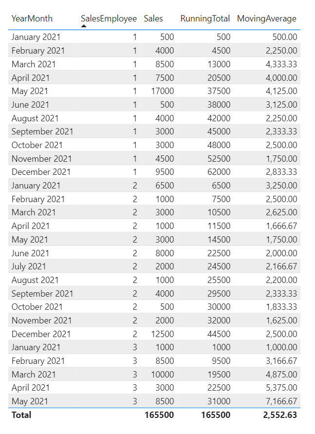
We need a measure that calculates the average of a rolling window, often also called moving average. In this example we’d like to return the rolling average sales per employee of the last three months.

Example:

The DAX for the measure:

MovingAverage = 
CALCULATE (
    AVERAGE (SalesTable[Sales] ),
    ALLEXCEPT ( 'SalesTable', SalesTable[SalesEmployee] ),
    DATESINPERIOD (
        'SalesTable'[YearMonth],
        STARTOFMONTH ( LASTDATE (  'SalesTable'[YearMonth] ) ),
        -3,
        MONTH
    )
)

Result:

Of course, you can also use SUM or other more advanced calculations for the rolling window.

The generic code:

Measure = 
CALCULATE (
    [Calulation: AVERAGE / SUM etc.] (Table[NumberColumn] ),
    ALLEXCEPT ( 'Table', Table[GroupingColumn] ),
    DATESINPERIOD (
        'Table'[DateColumn],
        STARTOFMONTH ( LASTDATE ( 'Table'[DateColumn] ) ),
        -[Number of Units for window],
        [Window: MONTH, YEAR, DAY]
    )
)

21. Count how many times a condition over a rolling window is met

We need a measure that calculates how many sales employees have had an average sales above 3000 over a rolling window of three months.

Example:

The DAX for the measure:

CountEmployeesAboveMovingAverage = 
CALCULATE ( 
    DISTINCTCOUNT ( SalesTable[SalesEmployee] ),
    FILTER (
        SalesTable,
        CALCULATE (
            AVERAGE (SalesTable[Sales] ),
            ALLEXCEPT ( 'SalesTable', SalesTable[SalesEmployee] ),
            DATESINPERIOD (
                'SalesTable'[YearMonth],
                STARTOFMONTH( LASTDATE (  'SalesTable'[YearMonth] ) ),
                -3,
                MONTH
            )
        ) > 3000
    )
)

Result:

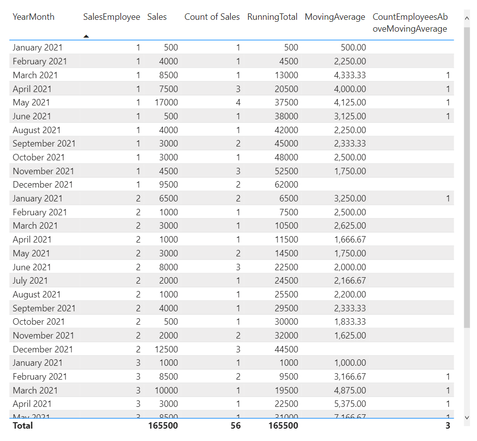
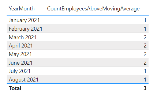
The first table shows per employee whether it fulfilled condition of having more than 3000 in average sales over the last three months, whereas the other table shows how many employees matched the condition per month.

The generic code:

Measure = 
CALCULATE ( 
    DISTINCTCOUNT ( Table[DinstinctCount/GroupingColumn] ),
    FILTER (
        Table,
        CALCULATE (
             [Calulation: AVERAGE / SUM etc.] (Table[NumberColumn] ),
             ALLEXCEPT ( 'Table', Table[GroupingColumn] ),
             DATESINPERIOD (
                   'Table'[DateColumn],
                    EOMONTH ( LASTDATE (  'Table'[DateColumn] ), 0),
                   -[Number of Units for window],
                    [Window: MONTH, YEAR, DAY]
             )
        ) > [threshold]
    )
)

22. How to retrieve the time from a datetime column

Here, we would like to parse out just the time from a datetime column.

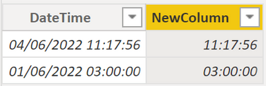
Example:

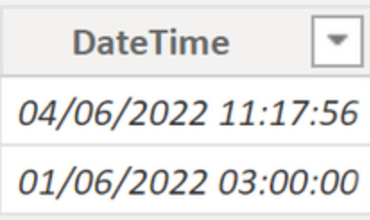
In this example, we are going to add a calculated column (right click on the column and click New Column):

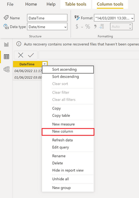
In the new column reference the old one:

NewColumn = TableDateTime[DateTime]

Finally, change the data type of the new column to Time:

Result:

tackytechtomMarch 26, 2022cheat sheetdax, power bi, power bi development 0

how to crack the mystery of the mighty DAX.

table of content.

1. Filter on the result of aggregate functions – “sql having clause”

2. Create ranks and indexes with calculated columns

3. Mark or get the second highest value or second latest date for a group

4. Get the max/min for a measure per group

5. Create ranks and indexes dynamically with measures

6. Find out the value appearing the most across several columns

7. Display values of large numbers with different unit abbreviations

8. Return the corresponding value for the max/min of a measure per group

9. Calculate the date difference between rows over the whole table or grouped by a status

10. Retrieve and display the value of the next row within a group

11. Grouping in DAX with AllExcept or ALL + Values – “sql group by clause”

12. Count rows meeting different conditions

13. Calculate the most frequent value in a column / return the top value for a certain measure

14. Show 0 instead of BLANKs in measure

15. Retrieve start of week date / end of week date

16. Check if values of one column exist in another column

17. Calculations with disconnected tables (without relationships)

18. Count occurrence of attributes per occurrence of another attribute (calculated table)

19. Create a Running Total measure

20. Create a rolling window / moving average measure

21. Count how many times a condition over a rolling window is met

22. How to retrieve the time from a datetime column

Leave A Comment Cancel reply