why the precedence of calculation groups is so important.

introduction.

Calculation groups is a powerful feature for data models in Analysis Service or Power BI Datasets (for an example, see this blog post). However, if you are planning to incorporate multiple calculation groups in one model, you should make sure to set the correct precedence for each calculation group. You might wonder what the precedence property is and why this is so important. Well, if you apply multiple calculation groups onto a measure i.e. in a matrix or due to a slicer, you need to control in which order the calculation groups shall be applied. Here, we explain this very relevant matter by an example.

plan of action.

1. The starting point
2. Divide and conquer
3. Showtime

1. The starting point

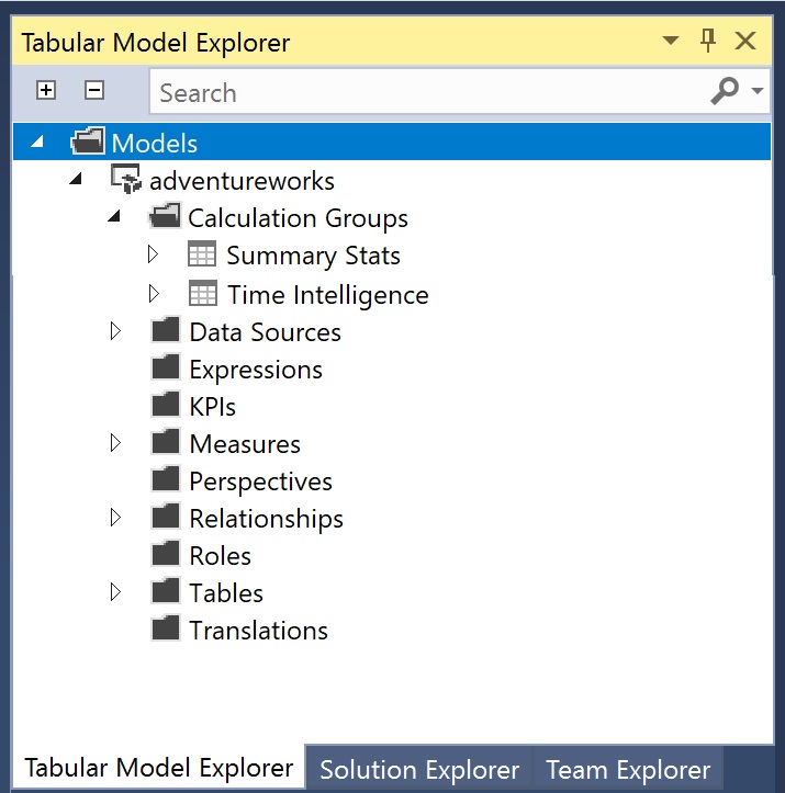
In our adventureworks model, we want to use two different calculation groups, summary stats and time intelligence:

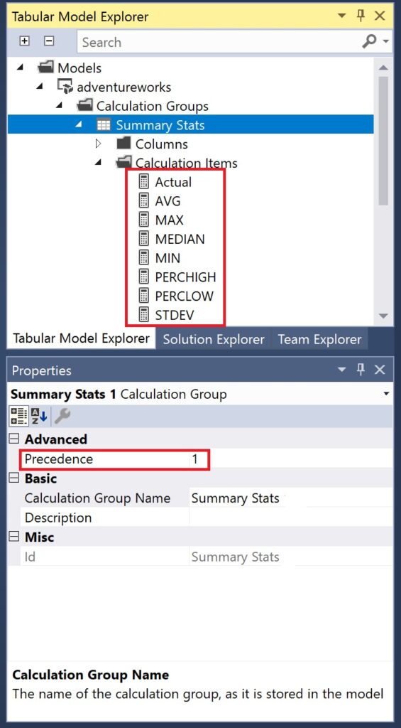
The summary stats calculation group applies various statistical functions onto the measure in charge:

The time intelligence calculation group on the other hand, deploys time functions onto the measure:

In both screenshots, the precedencies have been marked. But how do we decide on which value to use for each calculation group? The precedence property determines the application order of each calculation group. It requires an integer value that you can set as desired. A higher value means a higher priority, thus, this calculation group will be applied first. In our example, time intelligence has the higher precedence. So, if we happen to apply both groups onto a measure, the time function is evaluated prior the summary stats function.

2. Divide and conquer

To make it more tangible, let’s only consider the AVG member of the summary stats and the YTD member of the time intelligence:

AVG := CALCULATE ( AVERAGEX ( FactInternetSales, SELECTEDMEASURE() ) )

YTD := CALCULATE ( SELECTEDMEASURE(), DATESYTD ( 'DimDate'[DateKey] ) )

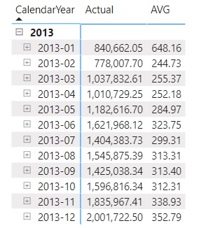
Before we start checking out how calculation groups behave with different precedencies, let’s have a closer look into our data:

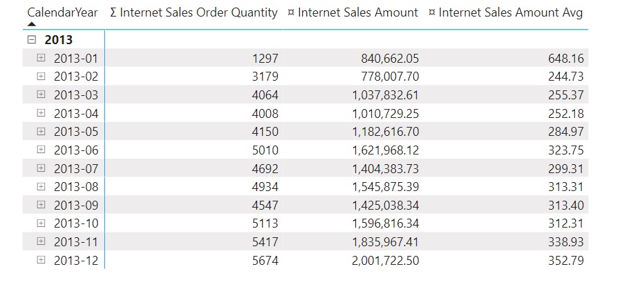
We can see historic internet sales data per month of the year 2013 with Order Quantity, Sales Amount and the Average Sales Amount per Order. To make it even more tangible, we will mostly focus on the month April, where there are 4008 Orders with Sales revenues of 1,010,729.25 leading to 252.18 average revenue per order.

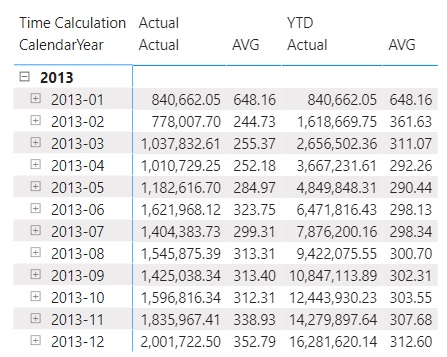
Now, let’s drag in the YTD member of the time intelligence group:

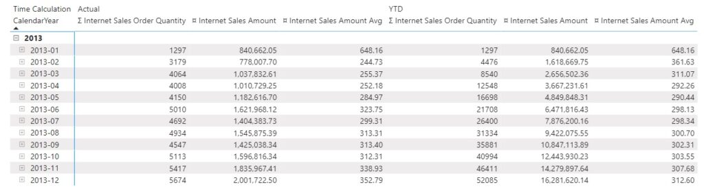
The YTD function helps to create a running total from January to the respective date. By April, we had 12548 Orders, with total sales revenue of 3,667,231.61, resulting in 292.26 average sales revenues per order (from January to April). So, DAX follows this logic to retrieve the values for Internet Sales Amount in the YTD context:

It uses a base measure (Note, this is not a member of the summary stats calculation group. It is a normal measure):
¤ Internet Sales Amount := SUM ( FactInternetSales[SalesAmount] )

It utilises the YTD member of the time intelligence calculation group:
YTD := CALCULATE ( SELECTEDMEASURE(), DATESYTD ( 'DimDate'[DateKey] ) )

So, DAX ends up performing this calculation:
CALCULATE ( [¤ Internet Sales Amount] ), DATESYTD ( 'DimDate'[DateKey] ) )

The order evaluation for the CALCULATE function in DAX is to first use the outer filter (in our case it’s the matrix applying a filter on each month), then the inner filter and finally apply the measure. In our April example (April = outer filter), we initially return all dates from 1st of January until 30th of April (YTD = inner filter), and then calculate the sum over this interval (¤ Internet Sales Amount).

In the next step, we wanna see how the AVG member of summary stats behaves when being combined with Internet Sales Amount:

Note, our AVG member from summary stats works just fine, since it returns the same values as the example above. Let’s go through the DAX logic here as well:

It uses the same base measure (“Actual” in the table graph above):
¤ Internet Sales Amount := SUM ( FactInternetSales[SalesAmount] )

It applies the AVG member of the summary stats calculation group:
AVG := CALCULATE ( AVERAGEX ( FactInternetSales, SELECTEDMEASURE() ) )

So, DAX ends up performing this calculation:
CALCULATE ( AVERAGEX ( FactInternetSales, [¤ Internet Sales Amount] ) )

Here we provide DAX with the FactInternetSales table. First the outer filter (the month from the matrix visual) is utilised, then DAX “sums” up the SalesAmount for each row over that table and stores all these rows. The sum function does not do anything here, as there is only one SalesAmount per row so just the SalesAmount for that row is returned. Finally, DAX calculates the mean over all stored rows. Obviously, an easier way to do the calculation would be to write this:

CALCULATE ( AVERAGE ( FactInternetSales[SalesAmount] ) )

However, we are using this more complex evaluation in the summary stats calculation group because this would work for any other measure of the table. Now the question is, what happens if we drag in both calculation groups into the matrix?

3. Showtime

We start with the precedence settings of 1 for summary stats and 2 for time intelligence meaning we first evaluate time intelligence members and then apply summary stats:

Considering the last column in particular, it looks decent and is in line with expectations as it displays the same values that we also derived in previous graphs. Still, let’s try to understand, what DAX has been done and how we ended up there.

Base measure:

¤ Internet Sales Amount := SUM ( FactInternetSales[SalesAmount] )

YTD:
YTD := CALCULATE ( SELECTEDMEASURE(), DATESYTD ( 'DimDate'[DateKey] ) )

AVG:
AVG := CALCULATE ( AVERAGEX ( FactInternetSales, SELECTEDMEASURE() ) )

Final DAX:
CALCULATE (
AVERAGEX ( FactInternetSales, [¤ Internet Sales Amount] )
),
DATESYTD ( 'DimDate'[DateKey] )
)

From the start, the outer filter (Date month) is applied, then DAX acknowledges the inner filter (YTD) due to its higher priority. For April, this means that the DATEYTD() function will directly change the context to use all dates from 1st January to the end of April. Afterwards, DAX determines the SalesAmount for each row with all the active filters in place (1st Jan – 30th April) and stores the outcome. Once it is done scanning the filtered table, it calculates the arithmetic mean (sum over all SalesAmounts and divide by the number of rows for the time interval 1st Jan – 30th April).
Great, the results seem correct, but what happens if we flip the precedencies of the two calculation groups? Well, let’s have a look on the next table graph:

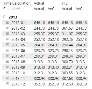
And here we can clearly see, why setting the right precedence is so important! The results of the very right column AVG do not make any sense or at least it’s not what we would have expected in the first place. What’s happened?

Base measure:
¤ Internet Sales Amount := SUM ( FactInternetSales[SalesAmount] )

AVG:
AVG := CALCULATE ( AVERAGEX ( FactInternetSales, SELECTEDMEASURE() ) )

YTD:
YTD := CALCULATE ( SELECTEDMEASURE(), DATESYTD ( 'DimDate'[DateKey] ) )

Final DAX:
CALCULATE (
AVERAGEX (
FactInternetSales,
CALCULATE ( [¤ Internet Sales Amount] ), DATESYTD ( 'DimDate'[DateKey] ) )
)
)

Same as always, it starts off with the outer filter (Date month). Thereafter, DAX iterates through each row of the filtered table which only contains rows for the selected month (i.e. April). DAX checks at first whether each row lays in the interval that has been calculated by the DATESYTD function (from 1th Jan – 30th April). Obviously, this is always the case, because our outer-filtered table only contains data from the selected month (April) in the first place. Long story short, the DATESYTD function does not really do anything here. Finally, DAX calculates the SalesAmounts for each row and stores them. When DAX reaches the end of the table, it calculates the average of that dataset and returns the result for that specific month, which in the end is the same as if there was no YTD function at all.

end.

I hope with this example, I was able to show what precedencies are and why they are so important. Admittedly, it is not that trivial to understand and it does get complicated quickly. My recommendation is to test different scenarios before you release a model with several calculation groups to production. Precedencies must be set correctly!